Visualising High-dimensional Data with R

Dianne Cook
Monash University

Session 1

Outline

time	topic
1:00-1:20	Introduction: What is high-dimensional data, why visualise and overview of methods
1:20-1:45	Basics of linear projections, and recognising high-d structure
1:45-2:30	Effectively reducing your data dimension, in association with non-linear dimension reduction
2:30-3:00	BREAK

Introduction

What is high-dimensional space?

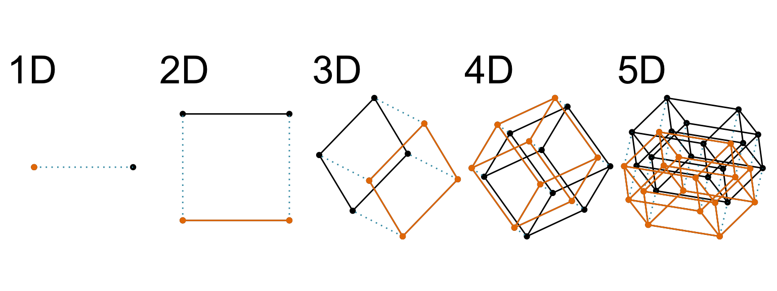
Increasing dimension adds an additional orthogonal axis.

If you want more high-dimensional shapes there is an R package, geozoo, which will generate cubes, spheres, simplices, mobius strips, torii, boy surface, klein bottles, cones, various polytopes, …

And read or watch Flatland: A Romance of Many Dimensions (1884) Edwin Abbott.

Notation: Data

\[\begin{eqnarray*} X_{~n\times p} = [X_{~1}~X_{~2}~\dots~X_{~p}]_{~n\times p} = \left[ \begin{array}{cccc} x_{~11} & x_{~12} & \dots & x_{~1p} \\ x_{~21} & x_{~22} & \dots & x_{~2p}\\ \vdots & \vdots & & \vdots \\ x_{~n1} & x_{~n2} & \dots & x_{~np} \end{array} \right]_{~n\times p} \end{eqnarray*}\]

Notation: Projection

\[\begin{eqnarray*} A_{~p\times d} = \left[ \begin{array}{cccc} a_{~11} & a_{~12} & \dots & a_{~1d} \\ a_{~21} & a_{~22} & \dots & a_{~2d}\\ \vdots & \vdots & & \vdots \\ a_{~p1} & a_{~p2} & \dots & a_{~pd} \end{array} \right]_{~p\times d} \end{eqnarray*}\]

Notation: Projected data

\[\begin{eqnarray*} Y_{~n\times d} = XA = \left[ \begin{array}{cccc} y_{~11} & y_{~12} & \dots & y_{~1d} \\ y_{~21} & y_{~22} & \dots & y_{~2d}\\ \vdots & \vdots & & \vdots \\ y_{~n1} & y_{~n2} & \dots & y_{~nd} \end{array} \right]_{~n\times d} \end{eqnarray*}\]

Why? (1/2)

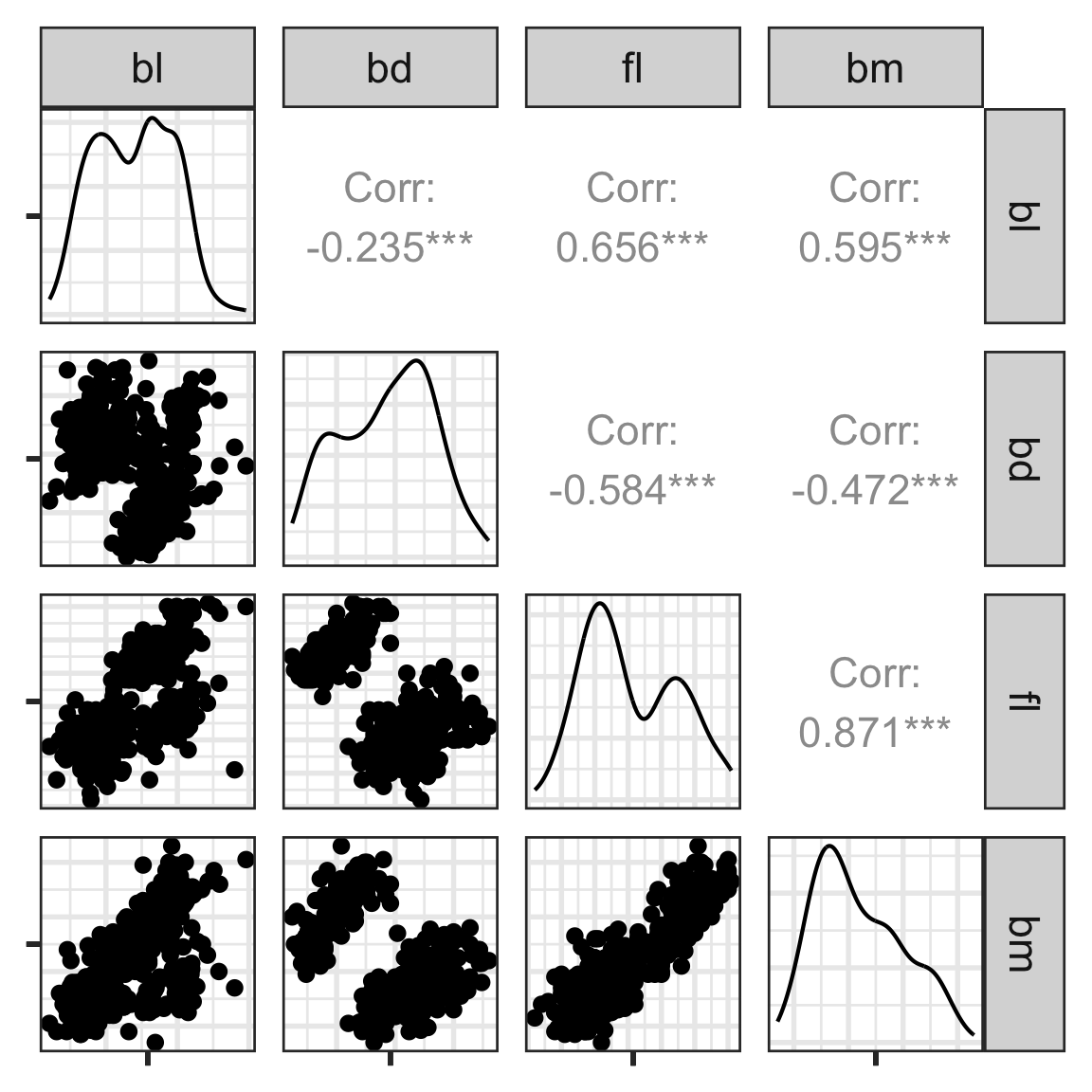
Scatterplot matrix

Here, we see linear association, clumping and clustering, potentially some outliers.

Why? (2/2)

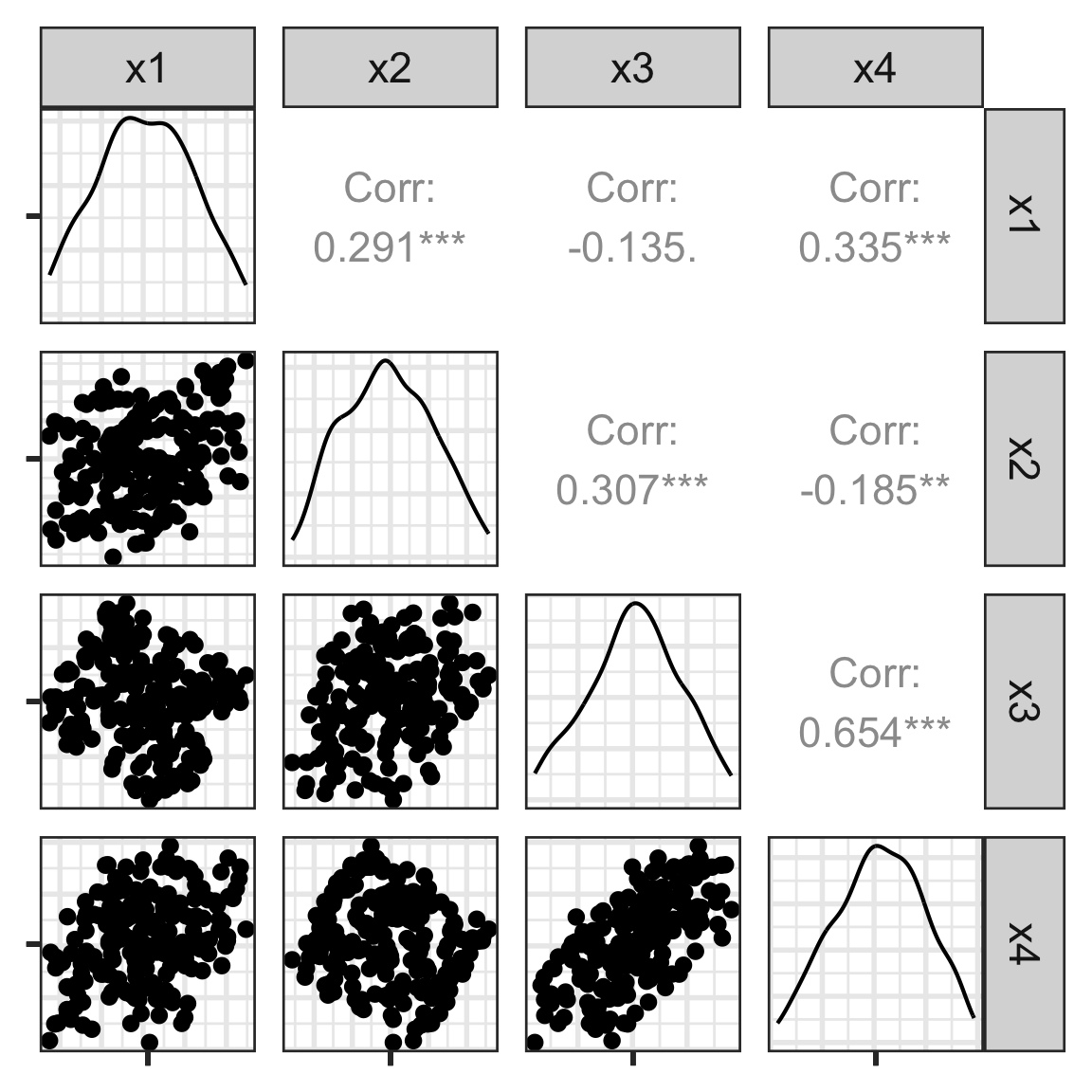
There is an outlier in the data on the right, like the one in the left, but it is hidden in a combination of variables. It’s not visible in any pair of variables.

And help to see the data as a whole

To avoid misinterpretation …

… see the bigger picture!

Image: Sketchplanations.

Tours of linear projections

Data is 2D: \(~~p=2\)

Projection is 1D: \(~~d=1\)

\[\begin{eqnarray*} A_{~2\times 1} = \left[ \begin{array}{c} a_{~11} \\ a_{~21}\\ \end{array} \right]_{~2\times 1} \end{eqnarray*}\]

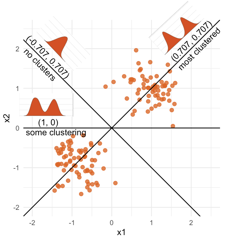
Notice that the values of \(A\) change between (-1, 1). All possible values being shown during the tour.

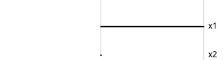
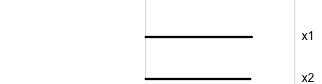
\[\begin{eqnarray*} A = \left[ \begin{array}{c} 1 \\ 0\\ \end{array} \right] ~~~~~~~~~~~~~~~~ A = \left[ \begin{array}{c} 0.7 \\ 0.7\\ \end{array} \right] ~~~~~~~~~~~~~~~~ A = \left[ \begin{array}{c} 0.7 \\ -0.7\\ \end{array} \right] \end{eqnarray*}\]

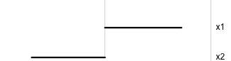
watching the 1D shadows we can see:

• unimodality
• bimodality, there are two clusters.

What does the 2D data look like? Can you sketch it?

Tours of linear projections

⟵
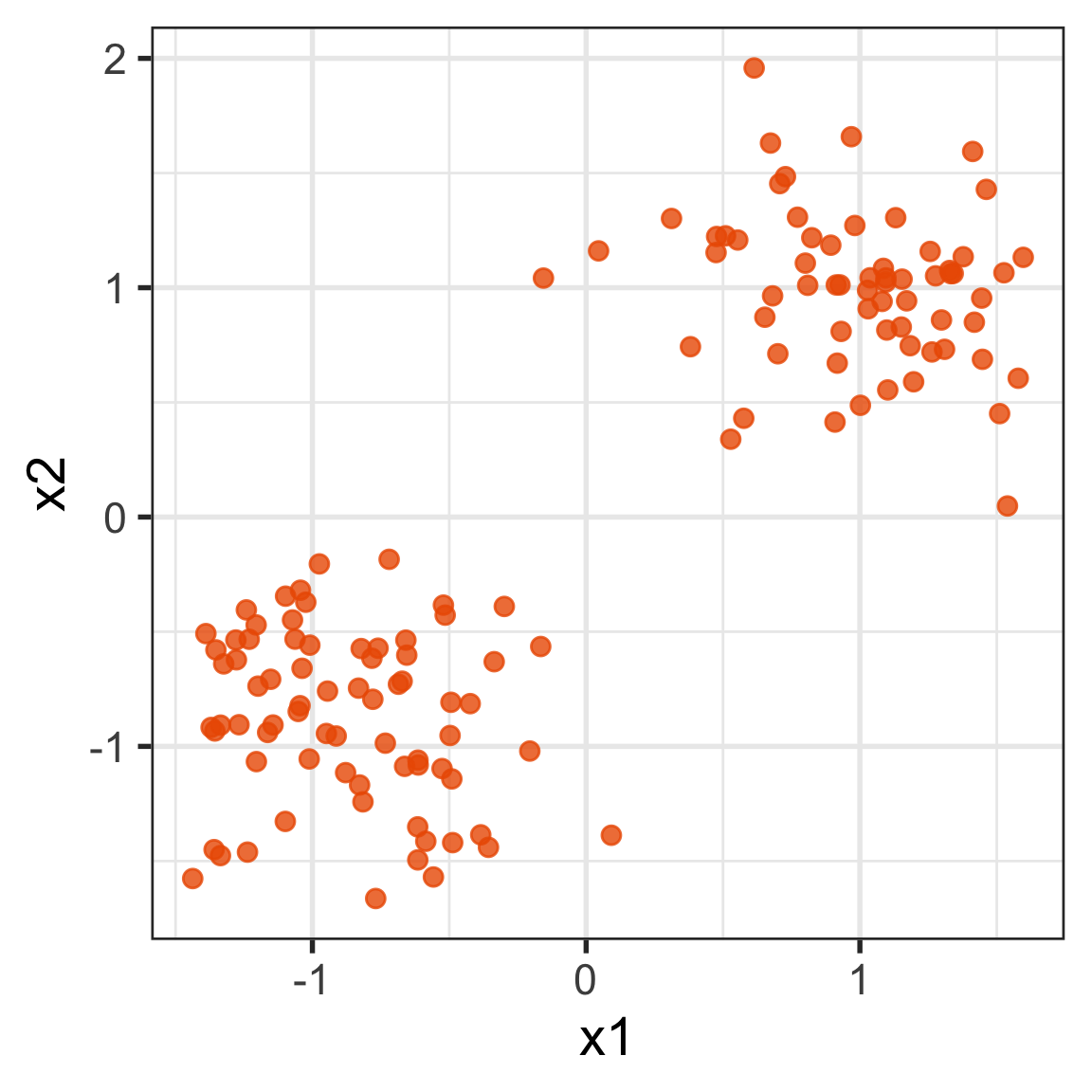
The 2D data

Tours of linear projections

Data is 3D: \(p=3\)

Projection is 2D: \(d=2\)

\[\begin{eqnarray*} A_{~3\times 2} = \left[ \begin{array}{cc} a_{~11} & a_{~12} \\ a_{~21} & a_{~22}\\ a_{~31} & a_{~32}\\ \end{array} \right]_{~3\times 2} \end{eqnarray*}\]

Notice that the values of \(A\) change between (-1, 1). All possible values being shown during the tour.

See:

• circular shapes
• some transparency, reveals middle
• hole in in some projections
• no clustering

Tours of linear projections

Data is 4D: \(p=4\)

Projection is 2D: \(d=2\)

\[\begin{eqnarray*} A_{~4\times 2} = \left[ \begin{array}{cc} a_{~11} & a_{~12} \\ a_{~21} & a_{~22}\\ a_{~31} & a_{~32}\\ a_{~41} & a_{~42}\\ \end{array} \right]_{~4\times 2} \end{eqnarray*}\]

How many clusters do you see?

• three, right?
• one separated, and two very close,
• and they each have an elliptical shape.

• do you also see an outlier or two?

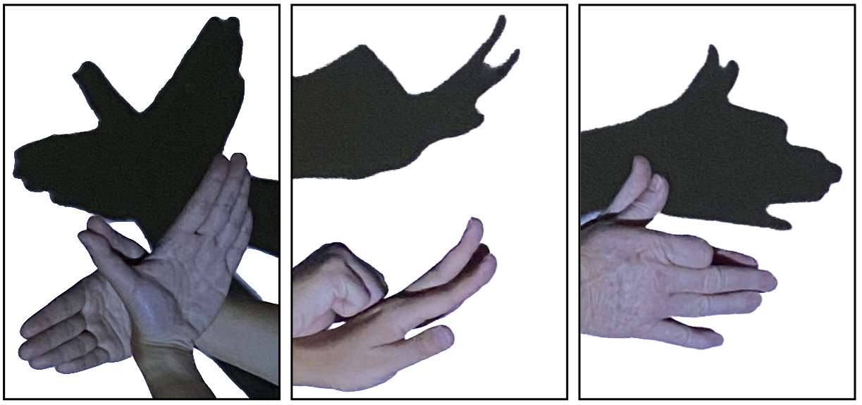
Intuitively, tours are like …

Anomaly is no longer hidden

Wait for it!

How to use a tour in R

This is a basic tour, which will run in your RStudio plot window.

library(tourr)
animate_xy(flea[, 1:6], rescale=TRUE)

This data has a class variable, species.

flea |> slice_head(n=3)

   species tars1 tars2 head aede1 aede2 aede3
1 Concinna   191   131   53   150    15   104
2 Concinna   185   134   50   147    13   105
3 Concinna   200   137   52   144    14   102

Use this to colour points with:

animate_xy(flea[, 1:6], 
           col = flea$species, 
           rescale=TRUE)

You can specifically guide the tour choice of projections using

animate_xy(flea[, 1:6], 
           tour_path = guided_tour(holes()), 
           col = flea$species, 
           rescale = TRUE, 
           sphere = TRUE)

and you can manually choose a variable to control with:

set.seed(915)
animate_xy(flea[, 1:6], 
           radial_tour(basis_random(6, 2), 
                       mvar = 6), 
           rescale = TRUE,
           col = flea$species)

How to save a tour

To save as an animated gif:

set.seed(645)
render_gif(penguins_sub[,1:4],
           grand_tour(),
           display_xy(col="#EC5C00",
             half_range=3.8, 
             axes="bottomleft", cex=2.5),
           gif_file = "gifs/penguins1.gif",
           apf = 1/60,
           frames = 1500,
           width = 500, 
           height = 400)

Your turn

Use a grand tour on the data set c1 in the mulgar package. What shapes do you see?

library(tourr)
library(mulgar)
animate_xy(c1)

Have a look at c3 or c7 also. How are the structures different.

05:00

Dimension reduction

What is dimensionality?

When an axis extends out of a direction where the points are collapsed, it means that this variable is partially responsible for the reduced dimension.

In high-dimensions

2D plane in 5D

3D plane in 5D

5D plane in 5D

Principal component analysis (PCA) will detect these dimensionalities.

Example: womens’ track records (1/3)

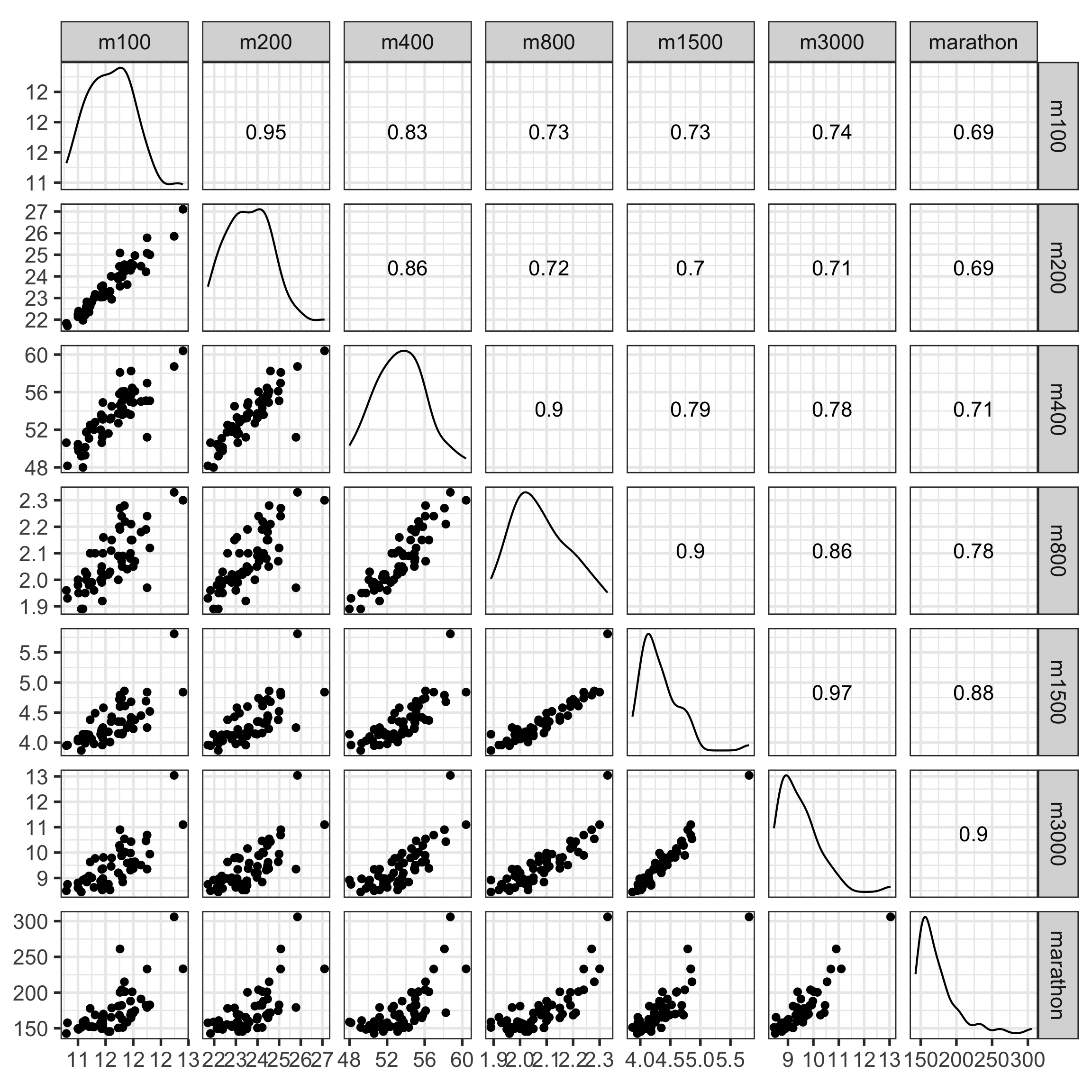
Source: Johnson and Wichern, Applied multivariate analysis

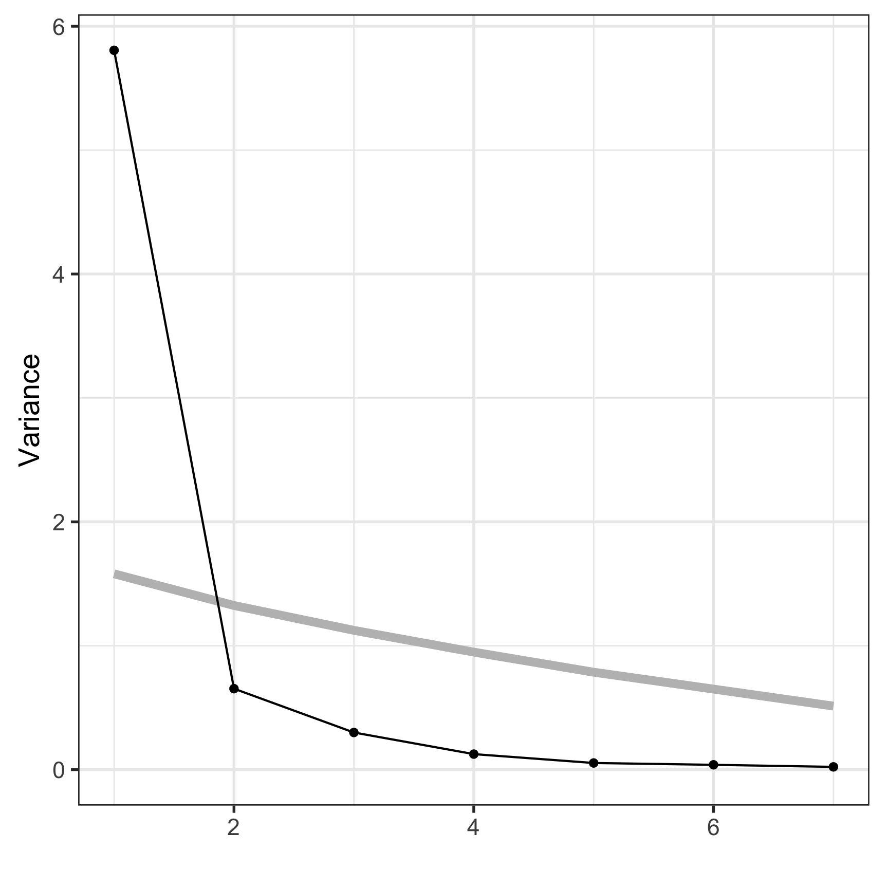
Example: PCA summary (2/3)

Variances/eigenvalues

[1] 5.806 0.654 0.300 0.125 0.054 0.039 0.022

Component coefficients

          PC1   PC2    PC3    PC4
m100     0.37  0.49 -0.286  0.319
m200     0.37  0.54 -0.230 -0.083
m400     0.38  0.25  0.515 -0.347
m800     0.38 -0.16  0.585 -0.042
m1500    0.39 -0.36  0.013  0.430
m3000    0.39 -0.35 -0.153  0.363
marathon 0.37 -0.37 -0.484 -0.672

How many PCs?

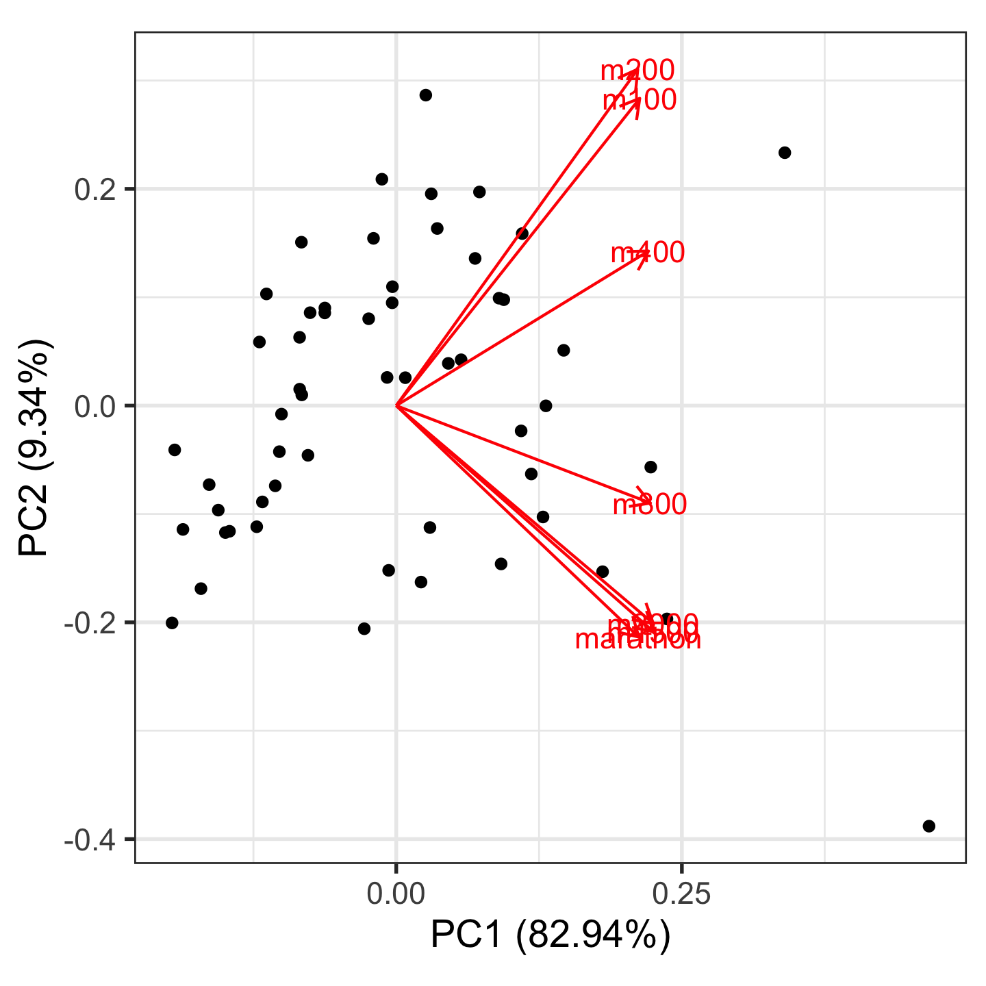
Example: Visualise (3/3)

Biplot: data in the model space

2D model in data space

track_model <- mulgar::pca_model(track_std_pca, d=2, s=2)
track_all <- rbind(track_model$points, track_std[,1:7])
animate_xy(track_all, edges=track_model$edges,
           edges.col="#E7950F", 
           edges.width=3, 
           axes="off")

Non-linear dimension reduction (1/2)

Find some low-dimensional layout of points which approximates the distance between points in high-dimensions, with the purpose being to have a useful representation that reveals high-dimensional patterns, like clusters.

Multidimensional scaling (MDS) is the original approach:

\[ \mbox{Stress}_D(x_1, ..., x_n) = \left(\sum_{i, j=1; i\neq j}^n (d_{ij} - d_k(i,j))^2\right)^{1/2} \] where \(D\) is an \(n\times n\) matrix of distances \((d_{ij})\) between all pairs of points, and \(d_k(i,j)\) is the distance between the points in the low-dimensional space.

PCA is a special case of MDS. The result from PCA is a linear projection, but generally MDS can provide some non-linear transformation.

Many variations being developed:

• t-stochastic neighbourhood embedding (t-SNE): compares interpoint distances with a standard probability distribution (eg \(t\)-distribution) to exaggerate local neighbourhood differences.
• uniform manifold approximation and projection (UMAP): compares the interpoint distances with what might be expected if the data was uniformly distributed in the high-dimensions.

NLDR can be useful but it can also make some misleading representations.

Non-linear dimension reduction (2/2)

UMAP 2D representation

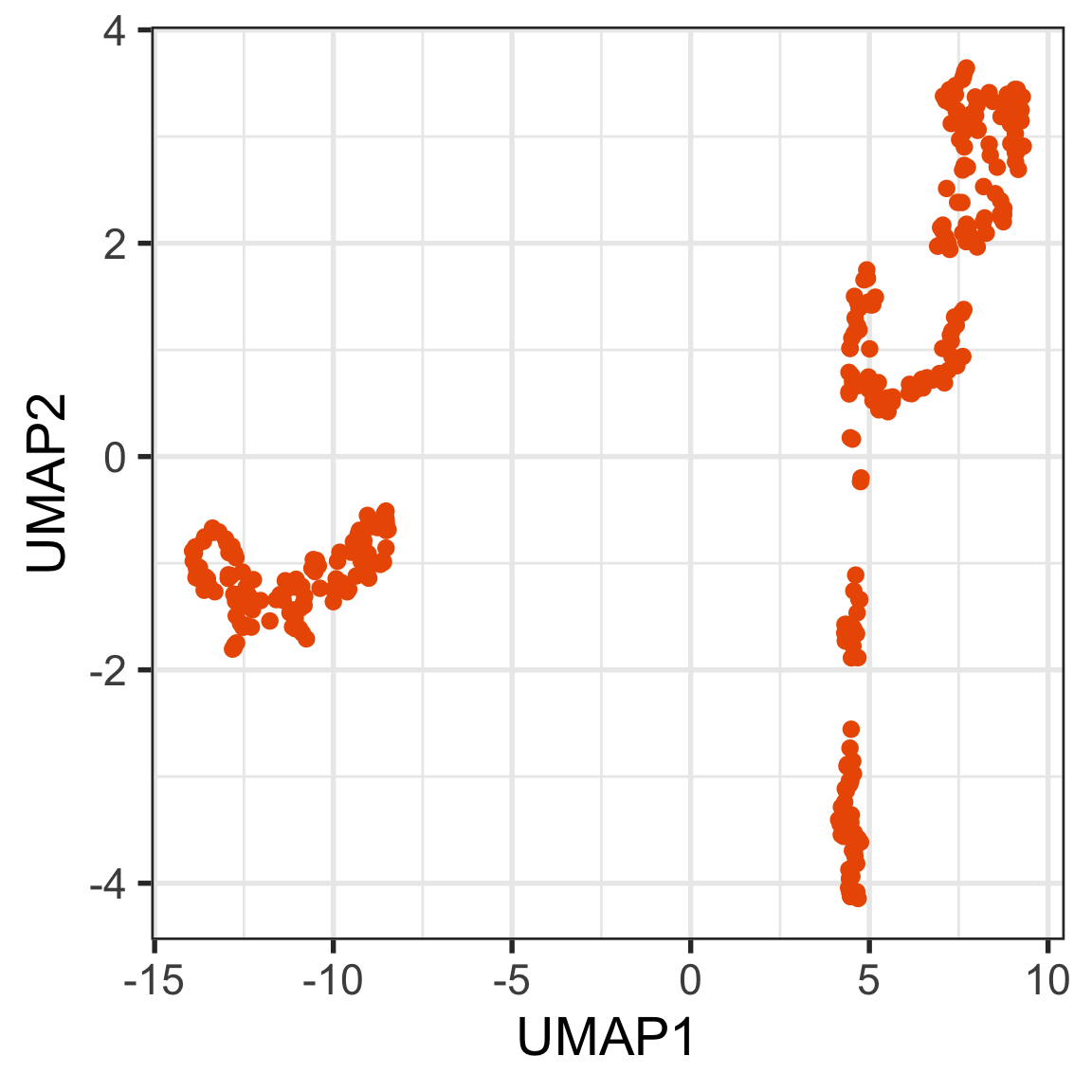
library(uwot)
set.seed(253)
p_tidy_umap <- umap(p_tidy_std[,2:5], init = "spca")

Tour animation of the same data

Your turn

Which is the best representation, t-SNE or UMAP, of this 9D data?

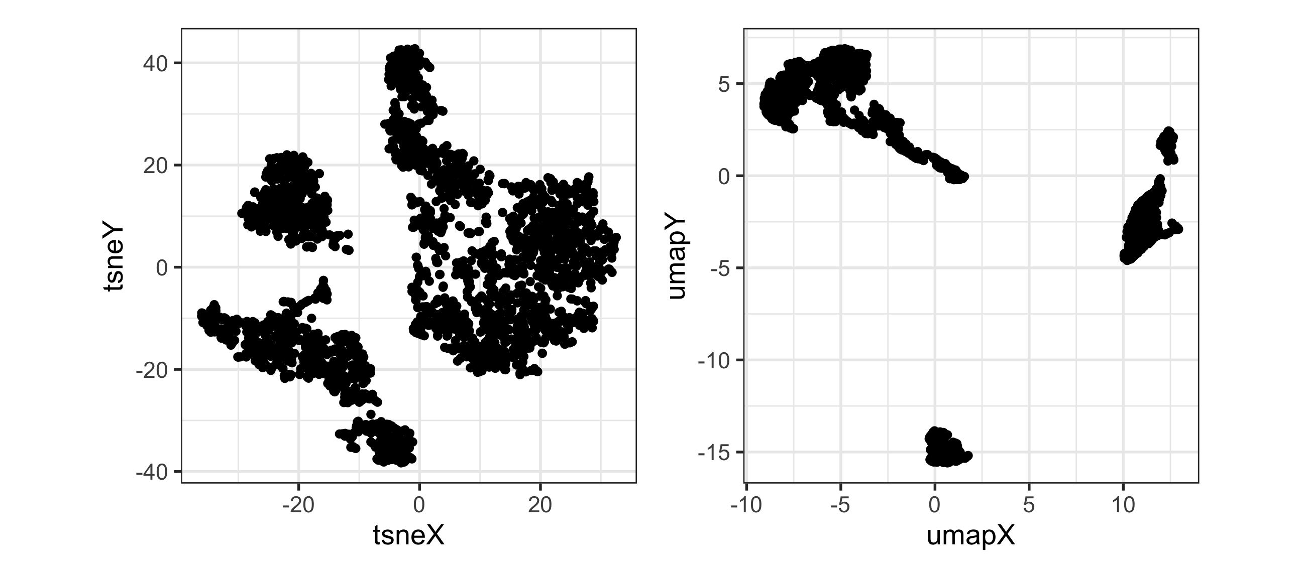
You can use this code to read the data and view in a tour:

pbmc <- readRDS("data/pbmc_pca_50.rds")
animate_xy(pbmc[,1:9])

05:00

Key conceptual points

• Avoid misinterpretation, by using your high-dimensional visualisation skills to look at the data as a whole.
• Examine model fit by by examining the model overlaid on the data, model-in-the-data-space. (Wickham et al (2015) Removing the Blindfold)

End of session 1

This work is licensed under a Creative Commons Attribution-ShareAlike 4.0 International License.