Di Cook Award: cassowaryr R-package tutorial

Harriet Mason

About

The cassowaryr package provides functions to compute scagnostics on pairs of numeric variables in a data set.

The term scagnostics refers to scatter plot diagnostics, originally described by John and Paul Tukey. This is a collection of techniques for automatically extracting interesting visual features from pairs of variables. This package is an implementation of graph theoretic scagnostics developed by Wilkinson, Anand, and Grossman (2005) in pure R and is designed to be easily integrated into a tidy data workflow.

The package’s primary use is as a step in exploratory data analysis, to give users an idea of the shape of their data and identify interesting pairwise relationships.

Installation

The package can be installed from CRAN using

install.packages("cassowaryr")

and from GitHub using

remotes::install_github("numbats/cassowaryr")

to install the development version.

Examples

Calculating the scagnostics

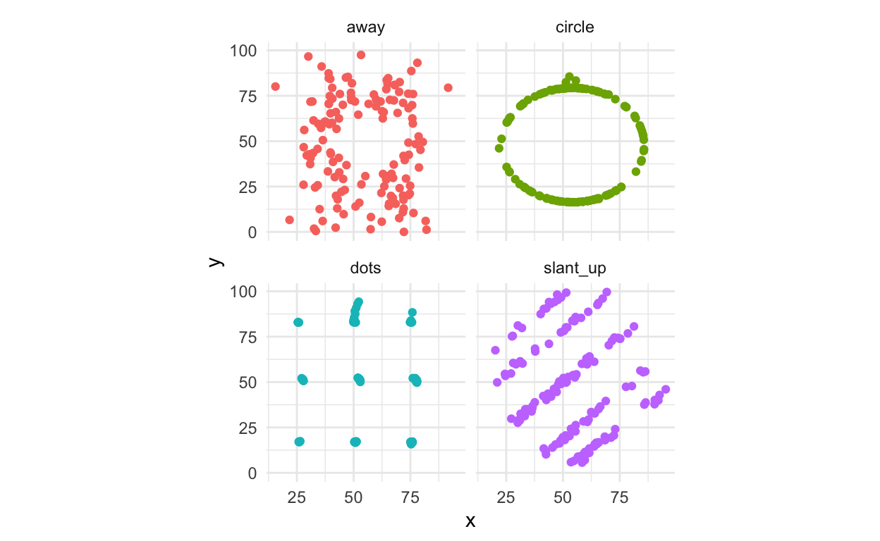
Here we will go through an example on the datasaurus dozen data (which comes loaded with the package). This data has several pairwise plots variables with the same mean, variance and correlation but strikingly different visual features. We will use a handful of these pairwise plots to show the best way to utilise the cassowaryr package. Here is a plot of the selected datasaurus dozen plots:

library(cassowaryr)
library(ggplot2)
library(dplyr)

# pick examples
exampledata <- datasaurus_dozen %>%
  filter(dataset %in% c("slant_up", "circle", "dots", "away"))


#plot them
exampledata %>%
  ggplot(aes(x=x,y=y, colour=dataset))+
  geom_point() +
  facet_wrap("dataset") +
  theme_minimal() +
  theme(legend.position = "none", aspect.ratio=1)

From a data frame, there are several ways to calculate scagnostics. If we simply have two variables we wish to calculate several scagnostics on, we use the calc_scags function and pass through the two variables as vectors.

calc_scags(exampledata$x, exampledata$y, scags=c("clumpy2", "convex", "striated2", "dcor")) %>%
  knitr::kable(digits=4, align="c")

striated2	clumpy2	convex	dcor
0.1853	0	0.7955	0.136

If instead we have a data frame with two variables and a grouping variable (a long form of a data set) then we can use the calc_scags function to get the scagnostics for each group.

longscags <- exampledata %>%
  group_by(dataset) %>%
  summarise(calc_scags(x, y, scags=c("clumpy2", "convex", "striated2", "dcor")))
longscags %>%
  knitr::kable(digits=4, align="c")

dataset	striated2	clumpy2	convex	dcor
away	0.0956	0.0000	0.7950	0.1326
circle	0.5255	0.0000	0.0117	0.2292
dots	0.1654	0.9932	0.0009	0.1266
slant_up	0.0942	0.8623	0.9145	0.1932

Finally, if we have a wide data set consisting of only numerical variables, we can use the calc_scags_wide to find the scagnostics on every pairwise combination of variables.

exampledata_wide <- datasaurus_dozen_wide[,c(1:2,5:6,9:10,17:18)]
widescags<- calc_scags_wide(exampledata_wide, scags=c("clumpy2", "convex", "striated2", "dcor"))
head(widescags, 4) %>%
  knitr::kable(digits=4, align="c")

Var1	Var2	striated2	clumpy2	convex	dcor
away_y	away_x	0.0956	0.0000	0.7950	0.1326
circle_x	away_x	0.1111	0.5222	0.8561	0.3839
circle_x	away_y	0.0857	0.2211	0.8642	0.1142
circle_y	away_x	0.1103	0.8403	0.7089	0.0818

Using the scagnostics

If the resulting scagnostic data set is small enough, we can find interesting scatter plots by simply looking at the table, however this is often not the case. If we want to find pairwise plots that are different to the others, we can find outliers on combinations of the scagnostics using an interactive scatter plot matrix (SPLOM). The code (but not the output) on how to do this is shown below:

library(GGally)
library(plotly)

splom_data <- widescags %>%
  ungroup() %>%
  mutate(lab = paste0(Var1, " , ", Var2)) %>%
  select(-c(Var1, Var2))

p <- ggpairs(splom_data, columns=c(1:4), aes(label=lab)) +
  theme_minimal()
ggplotly(p)

There are also a handful of functions that can summarise the scagnostic data. Using top_pairs allows us to find the top scagnostic for each pair of variables, while top_scags finds the top pair of variables for each scagnostic. Their usage is identical and shown below:

top_scags(widescags) %>%
  knitr::kable(digits=4, align="c")

Var1	Var2	scag	value
dots_y	circle_y	clumpy2	0.9948
slant_up_y	slant_up_x	convex	0.9145
slant_up_y	dots_y	dcor	0.9167
circle_y	circle_x	striated2	0.5255

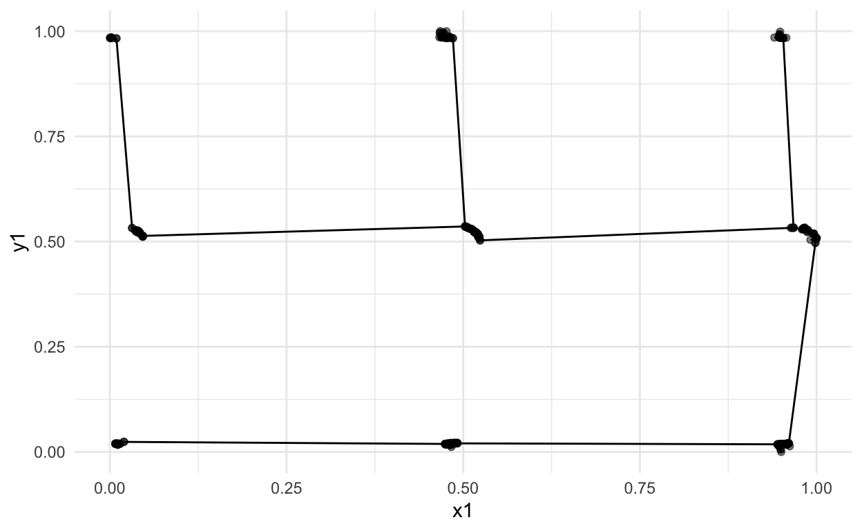
Diagnosing strange results

Occasionally we will get unexpected results for a scagnostic. To allow users to diagnose their own scagnostics, the package has several draw functions that will plot the graph based objects that were used to construct the measures. There is a draw function for the alpha hull, convex hull and MST. Below is an example of the MST function draw_mst.

drawexample <- exampledata %>%
  filter(dataset== "dots")

draw_mst(drawexample$x, drawexample$y, alpha=0.2) + theme_minimal()

cassowaryr R-package tutorial